A modern Central Processing Unit (CPU) consists of multiple independent execution units called cores. Each core is an independent hardware unit containing its own execution pipeline, registers, and control logic. A multicore CPU with $N$ physical cores can run up to $N$ independent execution streams in parallel.

Unlike physical cores, a thread is a software-defined execution context comprising a program counter, register states, and a call stack. Operating systems schedule threads onto physical cores. A core executes instructions from a single thread context at any given moment, unless it supports Simultaneous Multithreading (SMT).

SMT allows a single physical core to interleave instructions from multiple thread contexts, optimizing pipeline utilization without doubling raw execution hardware.

Parallel Execution

Parallelism arises from simultaneously executing workload(s) on multiple cores.

For $C$ physical cores and $T$ threads:

• If $T \le C$, threads can execute concurrently in parallel.
• If $T > C$, the operating system must time-slice execution.

In C++, multi-threading can be introduced via OpenMP directives or standard std::jthread/std::thread. While standard library threads provide low-level control, OpenMP simplifies thread pooling and work sharing with minimal developer overhead.

SMT allows multiple threads to share a single core, but this is a latency-hiding mechanism rather than a source of linear speedup.

Memory Hierarchy

The processor does not operate directly on data from main memory in most cases. Instead, it relies on a hierarchy:

• Registers (inside the core, fastest)
• L1 / L2 / L3 caches (on-chip, small but fast)
• Main memory (RAM)
• Secondary storage (SSD/HDD)

Data movement becomes progressively slower and more expensive as we go down this hierarchy.

For performance analysis, the critical boundary is between:

• on-chip computation
• off-chip memory (RAM)

Compute vs Data Movement

Any program performs two fundamental actions:

1. Compute - arithmetic operations executed by the core
2. Data movement - transferring data between memory and the core

Performance is limited by whichever of these becomes the bottleneck.

To quantify this, we define:

• Peak compute throughput: maximum operations per second a CPU can perform
• Memory bandwidth: maximum rate at which data can be transferred from memory

Arithmetic Intensity

Arithmetic intensity (AI) is the ratio of floating-point operations (FLOPs) to memory transfers (bytes) for a given kernel. It quantifies how many times each fetched byte is reused in computation; a higher AI implies more compute work per memory access.

This ratio categorizes kernels into two regimes:

• Low intensity → memory-bound
• High intensity → compute-bound

For example, the STREAM Triad benchmark (A[i] = B[i] + scalar * C[i]) measures sustainable memory bandwidth. Each iteration performs 2 FLOPs (one multiply, one add) but transfers 3 vectors’ worth of data (two reads, one write), totaling 24 bytes in double-precision. This yields an arithmetic intensity of approximately 0.083 FLOPs/byte, classifying it as a heavily memory-bound kernel.

Toward the Roofline Model

The roofline model was first introduced by a group of scientists at the University of California, Berkeley in 2008, in a paper titled:

Roofline: An Insightful Visual Performance Model for Floating-Point Programs 
and Multicore Architectures

By Samuel Williams, Andrew Waterman and David Patterson

The Roofline model combines peak compute throughput, memory bandwidth, and operational intensity to determine the maximum achievable performance of a program on a given machine. It answers two key questions:

• Is the program limited by compute or memory?
• How far is the implementation from hardware limits?

Building a Roofline Model

Constructing a Roofline model requires precise parameters. The accuracy of the model depends on the rigor of these measurements.

• Peak Sustained Memory Bandwidth: Measured using benchmarking suites like STREAM (specifically the Triad kernel). Refer to this implementation for detail.

• Peak Compute Throughput:

• Arithmetic Intensity:

• Arithmetic Intensity Ridge Point:

• The Roofline Bound:

Visualizing a Roofline Model

Here is the roofline model characterising the AMD Ryzen 5 6600H processor.

• X-axis: Arithmetic Intensity (log scale).
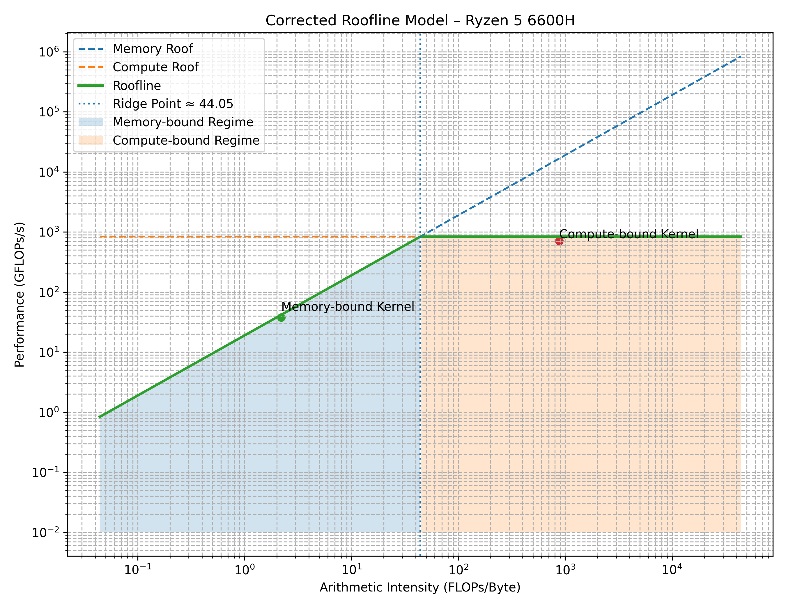
• Y-axis: Performance in FLOPs/sec (log scale).

Workloads fall into one of two operational regimes:

• Memory-Bound (blue): Performance is limited by and scales with memory bandwidth.
• Compute-Bound (orange): Performance is capped by the peak compute capacity of the execution units.

The upper boundary (plotted in green) represents the peak achievable performance as a function of Arithmetic Intensity (AI). The diagonal line represents the memory-bandwidth limit, and the horizontal ceiling represents the compute limit.

Using the Roofline Model

The Roofline model serves as a diagnostic tool, mapping workloads on a coordinate system to represent their execution behavior. The optimization goal is to increase arithmetic intensity, moving the workload to the right to saturate execution units and extract performance from the hardware.

• For memory-bound workloads: Increasing AI moves performance diagonally up the slope until it hits the compute ceiling.
• For compute-bound workloads: Performance is improved by optimizing execution efficiency (e.g., using SIMD vector instructions or reducing instruction overhead).

Glacier.HPC

Glacier.HPC focuses on profiling, benchmarking, and optimizing numerical kernels on consumer-grade hardware. Derived from the Glacier.ML codebase, this project focuses on:

• Measuring arithmetic intensity and raw performance.
• Constructing empirical Roofline models.
• Evaluating compiler and loop optimization strategies.

These insights are then used to optimize Glacier.ML.

To reference this post with full LaTeX equation formatting, you can view the raw markdown source at GitHub.

This post is based on experimental results from Glacier.HPC. A detailed analysis using the SAXPY kernel will be covered in the next post.

• SVM Classifier
• SVM Regressor

Both are implemented in C++ using:

• Eigen for linear algebra
• OpenMP for multithreading
• OpenBLAS for optimized BLAS routines

In local benchmarks, the classifier variant demonstrates 4–10× faster training compared to scikit-learn under comparable conditions. This post documents the algorithmic design, performance characteristics, and implementation philosophy behind these models.

Algorithmic Clarification: Not Classical Kernel SVM

Glacier’s SVM implementations are not dual-form, kernelized SVMs. Instead, they are based on:

PEGASOS
(Primal Estimated sub-Gradient Solver for SVM)

PEGASOS directly optimizes the primal objective using stochastic subgradient descent.

Classification Objective

Regression Objective (ε-insensitive loss)

Consequently, Glacier’s SVM variants are closer in behavior to linear stochastic gradient descent (SGDClassifier / SGDRegressor) rather than kernelized Support Vector Classifiers (SVC), as no feature mapping or kernel transformations are performed. The models are strictly linear.

Implementation Stack

1. Eigen + OpenBLAS

• Eigen provides matrix abstractions and expression templates.
• OpenBLAS accelerates low-level BLAS operations.

Key goals:

• Cache-friendly layouts
• Minimal heap allocations
• Efficient vectorized dot products
• Reduced abstraction overhead

The codebase avoids redundant temporary objects and prioritizes cache-local updates.

2. OpenMP Threading Strategy

Glacier defaults to using half of the available hardware threads. Limiting thread saturation mitigates thermal throttling, stabilizes sustained performance, and preserves overall system responsiveness. Because scikit-learn’s thread usage varies depending on the underlying BLAS backend, differences in thread policy can significantly impact comparative training times.

Performance Observations

Speed

The classifier model showed 4–10× faster training compared to scikit-learn in local tests.

Crucially, these comparisons are not strictly apples-to-apples due to differences in convergence criteria, memory layouts, and learning rate scheduling.

Underfitting on “Give Me Some Credit”

Both implementations underfit on the “Give Me Some Credit” dataset.

This is evidenced by poor recall on minority classes and overlapping confusion matrices. This occurs because the data requires a non-linear decision surface, which a strictly linear SVM cannot resolve without kernel expansion or feature engineering. This behavior is expected.

Architectural Decisions

Core design choices:

• Use primal optimization (PEGASOS)
• Avoid kernel complexity at this stage
• Emphasize hardware-level control
• Optimize CPU usage consciously
• Maintain explicit control over memory and threading

The codebase is not a direct transcription of any single reference; it is the result of iterative derivation, benchmarking, and refinement.

Learning with AI vs. Copying from AI

Mathematical derivations and implementation details were developed with the assistance of AI tools. The distinction between learning and copying lies in the ability to re-derive the objective function, implement the solver from scratch, and understand convergence behavior, regularization, and hardware trade-offs. Re-implementing a library from first principles guarantees conceptual ownership and clarity.

AI tools functioned as a refinement engine, error detector, and a resource to accelerate textbook research, while the core architectural decisions remained strictly manual.

Systems-Level Insights

Implementing PEGASOS from scratch highlights systems-level challenges like memory bandwidth limits, thread synchronization, numerical stability in subgradient descent, and learning rate scheduling. The exercise bridges algorithmic theory with hardware-aware optimization.

Future Scope

The next structural milestone is CUDA acceleration. This will enable:

• Large-scale mini-batch updates
• Faster convergence on high-dimensional datasets
• Experimental work in GPU-accelerated optimization

This work is planned for subsequent iterations.

Conclusion

Glacier’s SVM implementations leverage the PEGASOS primal optimization method in C++, integrating Eigen, OpenMP, and OpenBLAS to achieve high training speeds. They underfit predictably on non-linear datasets, reflecting expected theoretical limits.

The primary value of Glacier lies in establishing vertical control—bridging mathematical theory, memory layout, thread scheduling, and machine execution. This foundational understanding compounds.

This work shows that, when optimized systematically across mathematical, software, and hardware dimensions, kNN execution speed can be pushed closer to hardware limits, without modifying the underlying algorithm or target CPU.

By following a structured optimization path, the kNN Classifier and Regressor implementations achieve up to a 250x speedup over the naive baseline.

A Structured Path to Performance

The optimization followed a clear and layered progression:

1. Naive implementation of the mathematical model
2. Mathematical optimizations of the same model
3. Software-centric optimizations
4. Hardware-centric optimizations

Each layer presented their own bottlenecks and opportunities.

Mathematical optimizations

Efficient Selection of Neighbors

A significant portion of inference time is spent searching for the $k$ nearest neighbors. While a naive approach sorts or uses a std::priority_queue to retrieve the top elements, a more computationally efficient alternative uses std::nth_element to partition the vector in $O(N)$ average time.

Software-centric optimizations

Efficient Data Layout

• Contiguous Row-Major Representation: The 2D feature matrix, originally represented as nested vectors (std::vector<std::vector<float>>), was flattened into a contiguous 1D std::vector<float> using the mapping:

  X[row * num_cols + col]
  

  This flat layout offers:

• Reduced cache misses due to spatial locality.
• Predictable strided memory access.
• Enablement of compiler auto-vectorization (SIMD) on the contiguous memory block.

Hardware-centric optimizations

Parallelization using OpenMP

• Multithreading enables concurrent execution across CPU cores, reducing overall execution time despite minor synchronization overhead. Using OpenMP, this parallelization is enabled at compile time with the -fopenmp flag.
• On an AMD Ryzen 5 6600H CPU (6 cores, 12 threads), allocating half of the available hardware threads (6 threads) yielded the highest efficiency by avoiding hyperthreading overhead and thread contention.

SIMD Vectorization

• Distance computation relies heavily on sum reductions. Compiling with -march=native allows the compiler to leverage SIMD vector extensions (such as AVX2 or AVX-512) for automated reduction vectorization.

Compiler Flag Optimizations

• Switching from -O0 to -O3 enables aggressive compiler optimizations.
• -ffast-math permits additional optimizations (like reassociating floating-point operations) at the expense of strict IEEE 754 compliance, speeding up computations at the cost of strict numerical precision.

Profiling

• The perf utility was used to profile the executable and identify hot spots in the execution path.

Results

• Datasets ranged in size from $500 \times 10$ to $140,000 \times 10$.
• The optimized implementation achieved a $100\times$ to $250\times$ speedup compared to unoptimized baseline builds.
• The optimized implementation remains $4\times$ to $36\times$ slower than scikit-learn’s implementation under identical hyperparameters, demonstrating the sophistication of production-grade libraries.
• The optimization infrastructure introduced additional code complexity and increased compile times.

Benchmarking Setup

• Hardware: AMD Ryzen 5 6600H CPU, 8GB RAM.
• Environment: All manual background processes were closed, and the machine was set to performance power mode on AC power.

Key Learnings

• A clear distinction exists between a mathematical model on paper, a direct code translation, and a hardware-aware, optimized implementation.
• Understanding operating system scheduling and CPU cache hierarchies is critical for systems programming.
• Profiling tools (like perf) and integrated environments are essential for identifying micro-architectural bottlenecks.
• High-level libraries and wrappers abstract away significant underlying systems-engineering complexity.

The project originated as a practical follow-up to coursework in multivariate statistical modeling, specifically focusing on linear regression and its evaluation metrics. To translate theory into code, I used Stanford Online’s Statistical Learning lectures as a mathematical reference, building the logic without higher-level machine learning frameworks.

An initial prototype was reviewed by my artificial intelligence professor, whose feedback motivated me to expand the experiment into a more comprehensive library.

At present, Glacier.ML implements three stable models:

• Simple Linear Regression
• Multiple Linear Regression
• Binary Logistic Regression

The logistic regression implementation has been trained, tested, and validated on two real-world datasets:

• Pima Indians Diabetes Dataset (768 × 9)
• Wisconsin Diagnostic Breast Cancer Dataset (569 × 32)

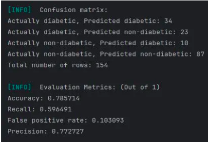
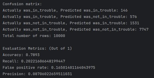
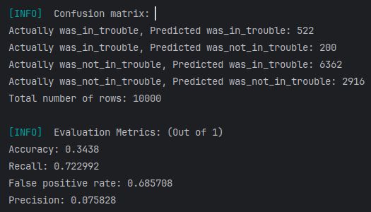
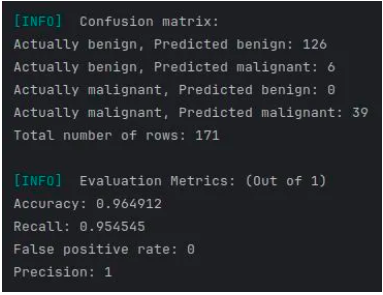
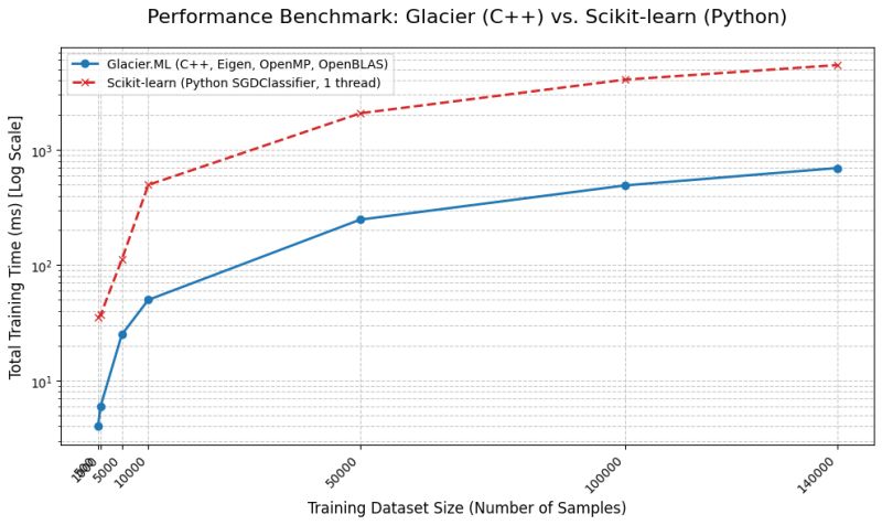
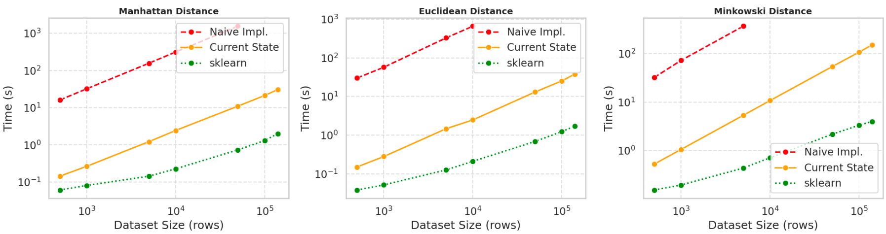
Confusion matrices for the datasets Pima Indians Diabetes Database and Wisconsin Cancer Diagnostic Dataset respectively Press enter or click to view image in full size

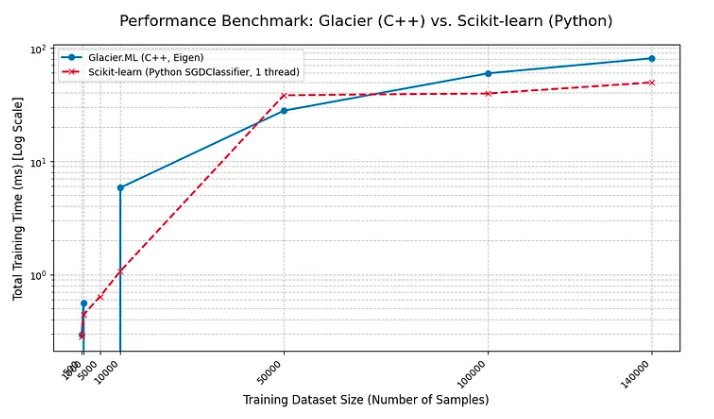
Benchmarking training time of Glacier’s Logistic Regression against Scikit-learn’s Logistic Regression Evaluation metrics and training times were benchmarked against scikit-learn’s logistic regression. Despite lacking explicit optimization and parallelism, Glacier.ML achieved comparable accuracy and training speed in these tests.

This implementation highlighted low-level numerical stability challenges, such as floating-point underflow, which are typically managed behind the scenes in higher-level ML libraries.

Below is a minimal example demonstrating dataset ingestion, training, prediction, and evaluation using Glacier.ML’s binary logistic regression pipeline.

#include "Glacier/Models/MLmodel.hpp"
#include "Glacier/Utils/utilities.hpp"

int main() {
    std::vector<std::vector<float>> X, X_t;
    std::vector<std::string> y, y_t;

    Glacier::Utils::read_csv_c("../Datasets/training_dataset.csv", X, y, true);
    Glacier::Utils::read_csv_c("../Datasets/testing_dataset.csv", X_t, y_t, true);

    std::vector<std::vector<float>> X_p = {
        {1, 2, 3 .... n}
    };
    std::vector<std::string> y_p = {"label_1"};

    Glacier::Models::MLmodel md(X, y);

    float hp1 = 1.0f;
    md.train(hp1);

    auto md_pred = md.predict(X_p);
    md.analyze_2_targets(X_t, y_t);

    return 0;
}

This example illustrates Glacier.ML’s core design goal: providing a minimal, explicit training and evaluation pipeline without hidden abstractions. Hyperparameters, data ingestion, and evaluation remain directly under user control.

The source code is available on GitHub.