Roofline Models: From Speculation to Modelling
Understanding the Machine
The device executing your program is built around a Central Processing Unit or CPU - a collection of independent execution engines called cores.
A core is a hardware unit capable of executing a sequence of instructions. It contains its own execution pipeline, registers, and control logic. Each core operates independently.
Modern processors contain multiple such cores. This is referred to as a multicore CPU. If a processor has (N) cores, it can execute up to (N) independent instruction streams in parallel.
A thread is not hardware. It is a software-defined execution context consisting of:
- a program counter
- a register state
- a stack
Threads are scheduled by the operating system onto cores. A core executes instructions from one thread at a time, unless it supports Simultaneous Multithreading (SMT).
In processors with SMT, a single core can maintain multiple thread contexts and issue instructions from them in an interleaved manner. This improves utilization of the core’s pipeline but does not double its computational capacity.
Parallel Execution
Parallelism arises from simultaneously executing workload(s) on multiple cores.
If there are:
- (C) cores
- (T) threads
Then:
- If (T <= C): threads can execute truly in parallel
- If (T > C): threads are time-sliced
In C/C++, OpenMP can be used to execute multithreading using its #pragma directives. Deeper,
fine-grained control can be harnessed using std::threads, although is much harder and results in
additional overhead, which OpenMP solves internally.
SMT allows multiple threads to share a single core, but this is a latency-hiding mechanism, not a source of linear speedup.
Memory Hierarchy
The processor does not operate directly on data from main memory in most cases. Instead, it relies on a hierarchy:
- Registers (inside the core, fastest)
- L1 / L2 / L3 caches (on-chip, small but fast)
- Main memory (RAM)
- Secondary storage (SSD/HDD)
Data movement becomes progressively slower and more expensive as we go down this hierarchy.
For performance analysis, the critical boundary is between:
- on-chip computation
- off-chip memory (RAM)
Compute vs Data Movement
Any program performs two fundamental actions:
- Compute - arithmetic operations executed by the core
- Data movement - transferring data between memory and the core
Performance is limited by whichever of these becomes the bottleneck.
To quantify this, we define:
- Peak compute throughput: maximum operations per second a CPU can perform
- Memory bandwidth: maximum rate at which data can be transferred from memory
Arithmetic Intensity
Arithmetic intensity is the ratio of compute operations to memory operations (Specifically FLOPs per byte transferred). As the name suggests, it helps quantify the number of times the fetched byte is used for computation. Hence, the program does more work per each memory access, thereby having a high arithmetic intensity.
The arithmetic intensity helps categorize a kernel into either of the two regimes:
- Low intensity → memory-bound
- High intensity → compute-bound
For example, the STREAM Triad benchmark (often just called “Triad”) measures sustainable memory bandwidth using a simple vector operation:
A[i] = B[i] + scalar * C[i]. Each iteration performs 2 FLOPs (one multiply and one add) but transfers 3 vectors’ worth of data (two reads and one write), typically 24 bytes for double precision. This gives an arithmetic intensity of about 0.083 FLOPs/byte, which is extremely low, making it a classic memory-bound kernel. Because of this, its performance is limited by memory bandwidth rather than compute, which is why it’s used to estimate peak sustained bandwidth in Roofline modeling.
The formula to calculate AI is defined in a section below.
Toward the Roofline Model
The roofline model was first introduced by a group of scientists at the University of California, Berkeley in 2008, in a paper titled:
Roofline: An Insightful Visual Performance Model for Floating-Point Programs
and Multicore Architectures

By Samuel Williams, Andrew Waterman and David Patterson
The roofline model combines:
- peak compute throughput
- memory bandwidth
- operational intensity
to determine the maximum achievable performance of a program on a given machine.
It provides a quantitative way to answer:
- Is the program limited by compute or memory?
- How far is it from hardware limits?
Building a Roofline Model
The following parameters are required to construct a roofline model. More rigorous the calculations, closer to truth is the roofline model.
- Peak Sustained Memory Bandwidth: Ideally using a memory bandwidth benchmarking suite.
Example - Triad from STREAM, published by Dr. John D McCalpin, University of Virginia.
(check out this article to see how Glacier.HPC used the TRIAD kernel to observe the peak sustained memory bandwidth)
- Peak Compute Throughput: Calculated using -
(Compute depends on many other factors like SIMD width among others)
- Arithmetic Intensity: Calculated using -
- Arithmetic Intensity Ridge Point: Calculated using -
- The Roofline Bound Calculated using the principal formula, also cited above -
Visualizing a Roofline Model
The original paper (cited above) demonstrates the roofline model on four different chipsets of its time. Here is the roofline model characterising AMD’s Ryzen 5 6600H processor.
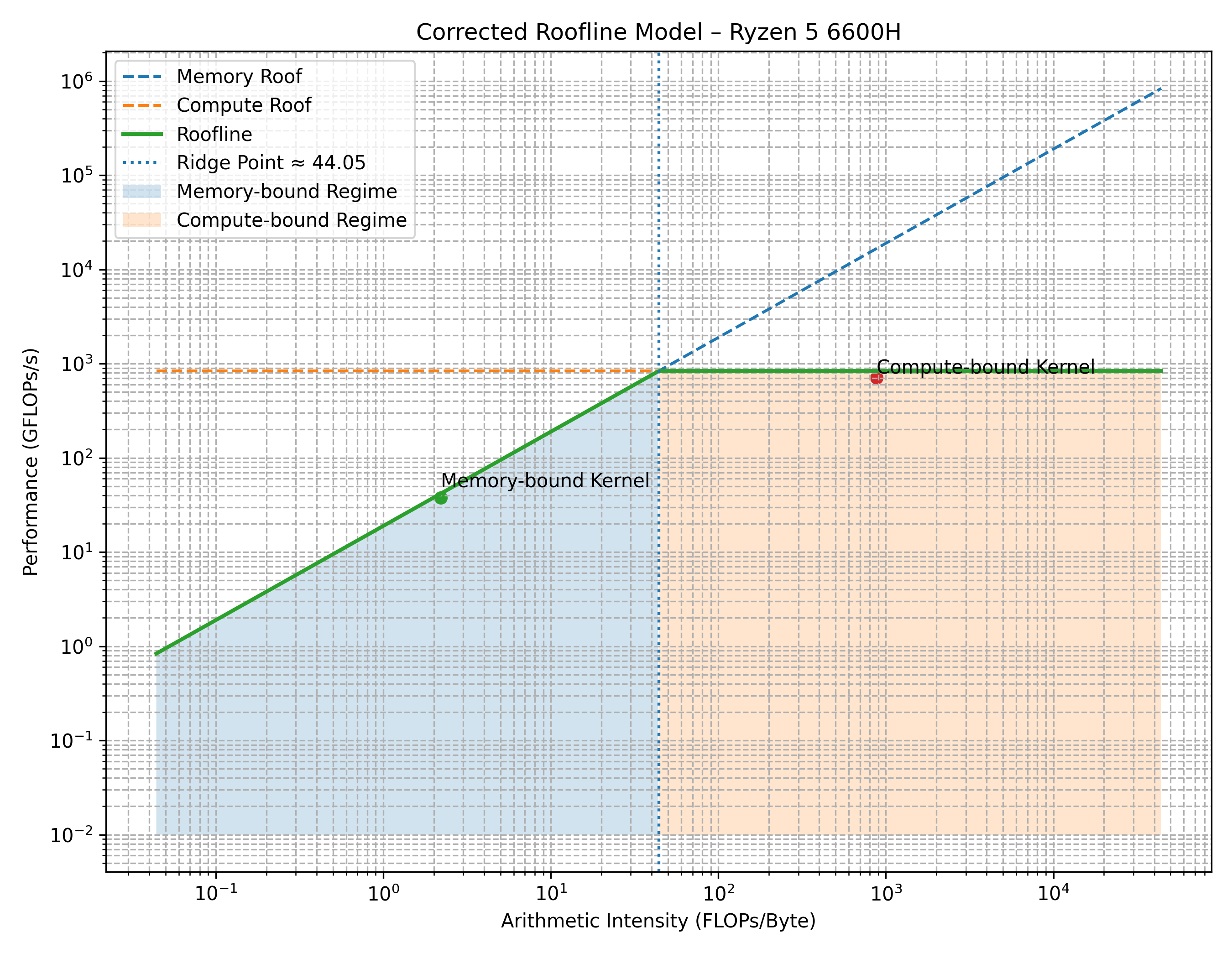
X-axis: Arithmetic Intensity on the log scale.
Y-axis: Performance (FLOPs/sec) on the log scale.
The roofline model is conceptually differentiated into two regimes, which all the workload inevitably fall into:
- Memory bound: (Represented in blue) The performance is bound and scaled with the memory bandwidth.
- Compute bound: (Represented in orange) The performance is capped by the peak compute capacity of the physical cores.
The green curve comprising of two straight lines represents the peak achievable performance
pertaining to the workload’s Arithmetic Intensity (hereby referred to as AI).
The diagonally placed line in green represents the Memory bound regime, whereas the
horizontally placed line in green represents the Compute bound regime.
Using the Roofline Model
The roofline model is a diagnostic of the workload’s nature. It merely places the workload on a coordinate system, which otherwise feels very abstract.
The goal remains to increase the workload’s AI, to push it as much to the right of the graph as possible. This ensures that the cores are increasingly saturated than before, thereby extracting more performance from the existing hardware.
- If memory bound (Represented using a green dot): As AI increases, the workload moves diagonally up along the green line, until it eventually plateaus along the horizontle line in green.
- If compute bound: (Represented using a blue dot) Performance is extracted by increasing the hardware’s compute efficiency, hence moving right along the horizontal line.
Glacier.HPC
Formally titled as
Glacier.HPC Profiling, Benchmarking and Analysis of Numerical Kernels derived from common Supervised Machine Learning
Algorithms on consumer grade computing hardware.
the project contains several iterative optimization experiments on numerical kernels, with their roofline plots and related discussions.
Glacier.HPC is derived from the author’s previous project Glacier.ML where ML numerical algorithms were implemented from scratch in C++. It focuses on:
- measuring arithmetic intensity, performance measures
- constructing roofline models
- evaluating optimization strategies to finally integrate the results into Glacier.ML.
If you wish to ask an AI model to explain the blog, rather copy-paste the original source code to include mathematical formulae from getting ignored: link
The content for this blog is derived out of the results obtained through experiments conducted in Glacier.HPC. A deeper discussion along with a concrete example using SAXPY will be explained in the upcoming blog.